Learning activity 1.1: Uniform motion and Newton’s first law

Introduction

Welcome to uniform motion and Newton’s first law. Take a couple of minutes to complete the following activity.

Let’s start with an experiment:

Move a toy car across a level surface at a constant speed. Now, imagine that you place an object on the top of the car. What will happen to the object if you suddenly stop the car?

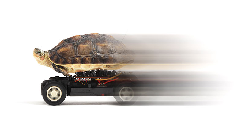
This lesson is about linear uniform motion. When an object is in linear uniform motion, it moves steadily in a straight line, always at the same speed and in the same direction. When you stop the car, the object on the top will remain at the same speed and direction. This is related to Newton’s first law of motion: “An object in motion will continue to move and an object at rest will remain at rest until some outside force acts on it.”

In this lesson, you will explore the basics of linear uniform motion and how uniform motion and Newton’s first law of motion are related, what causes motion, and how this all applies to real-world situations.

Acknowledgements (Opens in new window)

What you will learn

After completing this lesson, you will be able to:

solve problems involving uniform motion
conduct an investigation involving the motion of an object and its associated graph
draw and analyze motion graphs
use Newton’s first law to explain the motion of objects

Unit 1 Answer Sheet

You will have the opportunity to practice your skills through a variety of exercises. Check your solutions in “Answer Sheet for Unit 1 (Opens in new window)” after solving the exercises.

You will use the answer sheet for the next five lessons.

Velocity and displacement

In this lesson, you will explore kinematics, the study of motion, and dynamics, the study of the causes of motion and changes in motion.

When studying motion, you will encounter two different types of quantities: scalar quantities and vector quantities.

Note:

To indicate that a quantity is a vector, it will have a small arrow above the variable or letter (that is, symbol) for the quantity, like this: $\vec{d}$

A vector quantity’s direction, such as north [N], south [S], east [E], west [W], is indicated with square brackets.

In this lesson, you will analyze three vector quantities: displacement, velocity, and force. See “Comparison of Scalar and Vector Quantities (Opens in new window)” for a summary of the properties of some of the most common vector and scalar quantities.

Press each term below for more details and examples.

Scalar quantities

A scalar quantity has magnitude (size) and units only, but no direction.

Four clocks showing 15s, 30s, 45s, and 60s.

time is a scalar

Examples of scalar quantities are time, area, volume, temperature, and mass.

Vector quantities

A vector quantity has a magnitude (size) and units as well as a direction.

Road and yellow arrow illustrating speed.

Examples of vector quantities are displacement, velocity, force, and acceleration.

Distance vs displacement

Activity

Let’s start by analyzing the difference between distance, a scalar quantity, and displacement, a vector quantity.

Distance is the length of the path taken and is usually measured in metres or kilometres.

Displacement represents the change in position in a given direction.

After finishing this activity, you will have a better understanding of these concepts, which will be further detailed in the rest of the lesson.

See “Distance vs. displacement simulation”, (Opens in new window) execute the simulation, and solve the suggested challenges.

Start

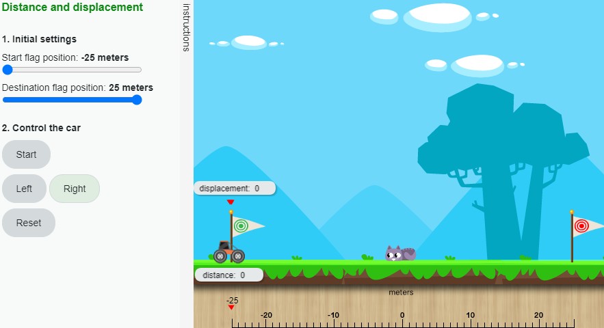
Press Enter here for an accessible version of Distance and displacement. (Opens in new window)

Press the name of each concept to view its definition.

Distance

Distance is the length of the path taken and is usually measured in metres or kilometres.

Displacement

Displacement ( $\vec{∆ d}$ ) is a vector quantity that represents the change in position in a given direction. In other words, displacement indicates the size of the change and its direction.

The symbol for displacement is $\vec{∆ d}$ , where the Greek letter Δ (delta) means change. Displacement is usually measured in metres (m) or kilometres (km) and the direction should be shown in square brackets.

When an object travels in a straight line in only one direction the magnitude (size) of the displacement is equal to the magnitude of the distance.

In this course, however, you will work with displacement since it provides more information about the movement (motion) than distance does.

To find displacement using positions, use the following equation:

Displacement’s general equation

$\vec{∆ d} = \vec{d_{2}} - \vec{d_{1}}$ .

Where:

$\vec{d_{2}}$ is the final position.

$\vec{d_{1}}$ is the initial position.

This means that the change in position or displacement is equal to the second position minus the first position.

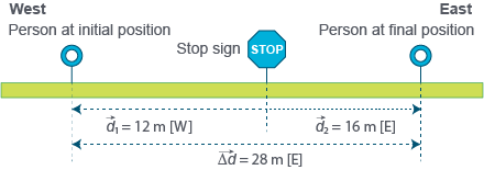
Example: Displacement of a person walking

A person starts walking from an initial position $\vec{d_{1}} = 12 m [W]$ of a stop sign to a final position of $\vec{d_{2}} = 16 m [E]$ of the same stop sign. Calculate the displacement.

Displacement by looking at initial and final positions

The advantage of using the equation is that you don’t have to draw or look at the diagrams to find the displacement.

Press the following button to display the suggested answer.

As you can see in the following diagram, the person first moves 12 m east to the stop sign and then another 16 m away from it for a total of 28 m toward the east. This means the displacement is $\vec{∆ d} = 28 m [E]$

In other words, we have:

$\vec{d_{1}} = 12 m [W]$

$\vec{d_{2}} = 16 m [E]$

Using the formula:

$\vec{∆ d} = \vec{d_{2}} - \vec{d_{1}}$

$\vec{∆ d} = 16 - (- 12)$

$\vec{∆ d} = 28$

This means that the change in position or displacement is equal to the second position minus the first position.

Velocity

When you know the displacement of an object and the time it took, you can find the velocity.

The velocity of an object is the rate at which the position is changing with respect to time.

Like displacement, velocity is another vector quantity so it must always have a direction. Its direction will match the direction of the displacement in the equation you are about to learn.

To find the velocity of an object, divide displacement by time using the following equation:

\vec{v} = \frac{\vec{∆ d}}{∆ t}

Where:

$\vec{v}$ is the velocity (in m/s or km/h), which is a vector quantity
$\vec{∆ d}$ is the displacement (in m or km), which is a vector quantity
$∆ t$ is the time (in s or h), which is a scalar quantity

The following sample problem will help you practice using this equation.

Example: Finding the velocity of a train

Find the velocity of a train that moves 126 km [W] in 2.0 hours.

Press the following button to display the suggested answer.

Given:

$\vec{∆ d} = 126 k m [W], ∆ t = 2.0 h$

${\vec{v}}_{} = \frac{\vec{∆ d}}{∆ t}$

${\vec{v}}_{} = \frac{126 km [W]}{2.0 h}$

${\vec{v}}_{} = \frac{63 km}{h} [W]$

The train moves at 63 km/h [W]. Note that the direction (west) of the velocity matches that of the displacement.

In this problem, the train moves quite far over a long period of time. It is unlikely that it moves at exactly this velocity for the entire two hours. More likely, this is an average velocity for the train during this time period. In this lesson, velocity will be assumed to be average unless described otherwise.

There is another term for the velocity at a particular moment (or instant) in time. It’s called the instantaneous velocity and is measured by devices such as speedometers and radar guns used by police. You will learn more about instantaneous velocity later in this course.

Exercises: Displacement and velocity

Screen reader users: use the displacement formula to answer the following questions.

1. Find the displacement for each of the following. Use the simulation to verify your answers.

$\vec{d_{1}} = 22 m [E], \vec{d_{2}} = 36 m [E]$
$\vec{d_{1}} = 32 m [W], \vec{d_{2}} = 14 m [W]$
$\vec{d_{1}} = 52 m [N], \vec{d_{2}} = 15 m [S]$

2. A storm is moving at an average velocity of 4.6 km/h [E] toward your town, which is 23 km [E] away. How long will it take the storm to reach the town?

Start

Understanding checkpoint

Motion Graphs

Building a velocity graph

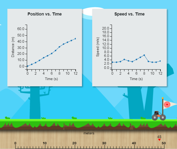
In this lesson, we will discuss motion and its visual representations. Graphs will be used to demonstrate how motion is represented and will give you a better idea of how an object is moving. Let’s start creating your first graphs.

See “Instructions of the activity (Opens in new window)” and use the “blank graph paper (Opens in new window)” to execute the simulation and solve the suggested challenges.

Start

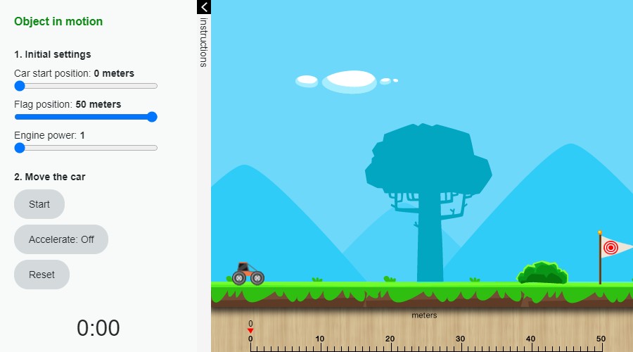
Press Enter here for an accessible version of Object in motion. (Opens in new window)

Congratulations! You just created your first position-time and velocity-time graphs.

The following example is a possible solution to the activity.

Can you identify the differences between the graphs? Next, we will analyze these types of graphs with regard to constant velocity.

Illustration showing plotting a position-time and a velocity-time graph.

Position-time graphs

When the position increases at a constant rate (constant velocity), the graph displays an inclined line. The following position-time graph represents the velocity of the object in motion with constant velocity.

Time (s)	Position (m) [E]	$\vec{d}$
0	0	d₁
2	10	d₂
4	20	d₃
6	30	d₄
8	40	d₅
10	50	d₆

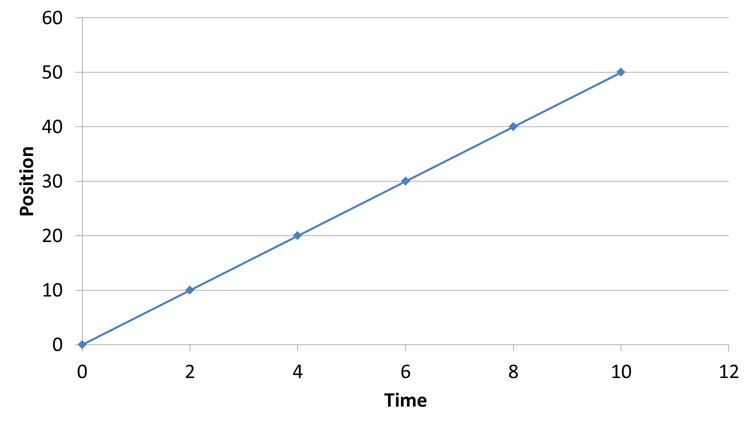
Line graph with time from 0 to 10 and position rising in a straight line from 0 to 50

Let’s analyze the graph in detail. The slope is the key element that you should consider to understand the behaviour of the object in motion. Its analysis will provide information about the velocity and behaviour of the object.

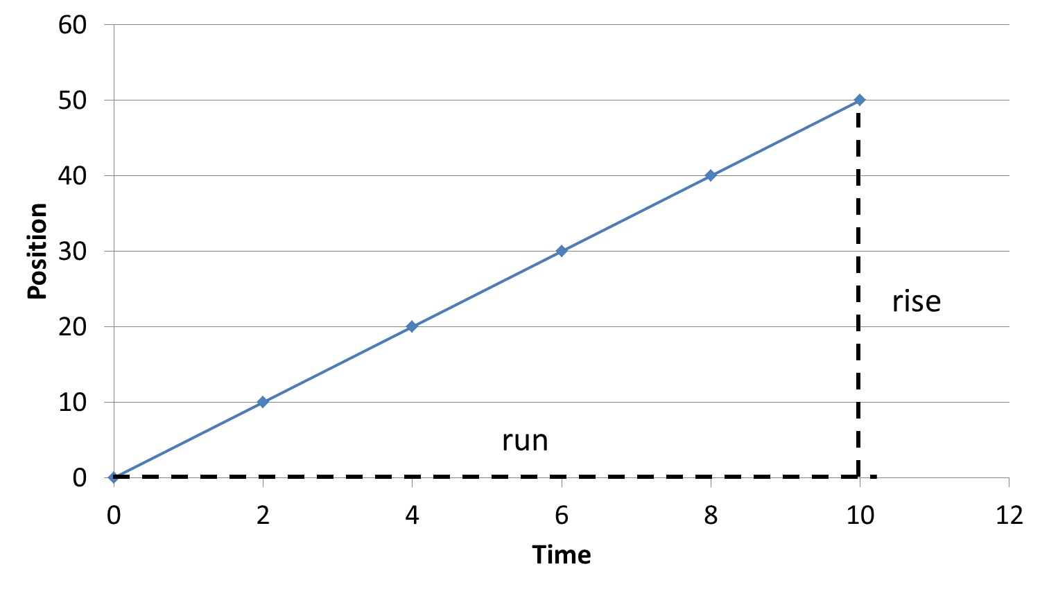
The same line graph, with horizontal run of 10 and vertical rise of 50 highlighted

Press each of the following terms to learn more about the graph.

Slope

The slope (represented by m) of a line is defined as “rise over run.” In other words, slope is equal to the vertical rise divided by the horizontal run between two points on a line. For example, if you check the point 10s, you may notice that the rise is 50m.

Now, let’s put the rise and run numbers and units into the slope equation as follows:

$s l o p e = \frac{r i s e}{r u n}$

$m = \frac{50 m [E]}{10 s}$

$m = 5.0 \frac{m}{s} [E]$

Calculating velocity

Now, using the same data, let’s calculate the average velocity of the object.

$\vec{v} = \frac{\vec{∆ d}}{∆ t}$

$\vec{v} = \frac{50 m [E]}{10 s}$

$\vec{v} = 5.0 \frac{m}{s} [E]$

You can see that the slope of the line is the same as the velocity of the object, so
$s l o p e = m = \frac{r i s e}{r u n} = \frac{\vec{∆ d}}{∆ t} = v = v e l o c i t y$

In other words, velocity is the change in position (always the vertical rise on a graph) divided by the time (always the horizontal run on a graph). The slope of a position-time graph is the velocity.

Uniform motion

You might also see that this straight-line graph shows that the moving object always covers the same distance in the same time interval, when this happens it’s because an object has uniform motion. That means that the object always covers the same distance in the same time interval.

Velocity-time graphs

Since the object in motion has uniform linear motion, the velocity is constant at all times. Remember the graphs that you created in the previous activity? You also drew a different type of motion graph: a velocity-time graph.

Let’s analyze the following graph as an example:

Uniform motion

As you can see, this graph shows that the object is moving with uniform motion. The velocity is constant at 5 m/s [E], as shown by the horizontal line that does not deviate from its level at all.

Displacement

Now, pay attention to the area of the rectangle that’s outlined by the velocity line at 5 m/s [E] and the time period from 0 to 10 s on the time axis (this is the shaded region shown on the graph). The area provides other relevant information about the movement.

You can notice that the area (50m) is also the displacement of the object. As you can see, the length of the rectangle is the time span, and the width of the rectangle is the velocity.

Calculating displacement

You’ve already seen that if you multiply velocity by the time interval, you get the displacement. So let’s confirm our numbers:

$\vec{∆ d} = \vec{v_{a v g}} x ∆ t$

$= 5.0 \frac{m}{s} [E] x 10 s = 50 m[E]$

Now you know that the area outlined on a velocity-time graph by the velocity line and the time axis is equal to the total displacement of the object. You can use this rule to get total displacement from a velocity-time graph. The area between a velocity line and the time axis is the total displacement.

Activity

To further understand position-time and velocity-time graphs, execute the following simulation.

As you can see, it is the same simulation as in the previous activity, but now you can visualize the motion of the car.

Try different configurations and see how the movement of the car is represented in a visual way.

Start

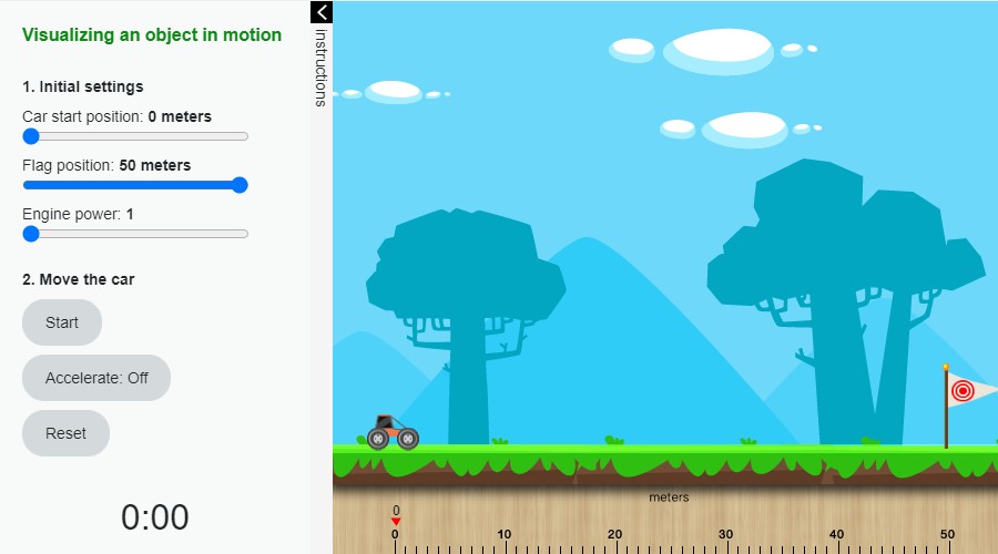
Visualizing an object in motion

Now that you understand the importance of visualizing motion through graphs, it is also important to be aware of some conventions that will be followed in this course. Please review and familiarize yourself with the “conventions to construct graphs (Opens in new window)”.

The next example will help you practice your graphing skills, as well as give you an opportunity to find velocity and displacement by examining motion graphs.

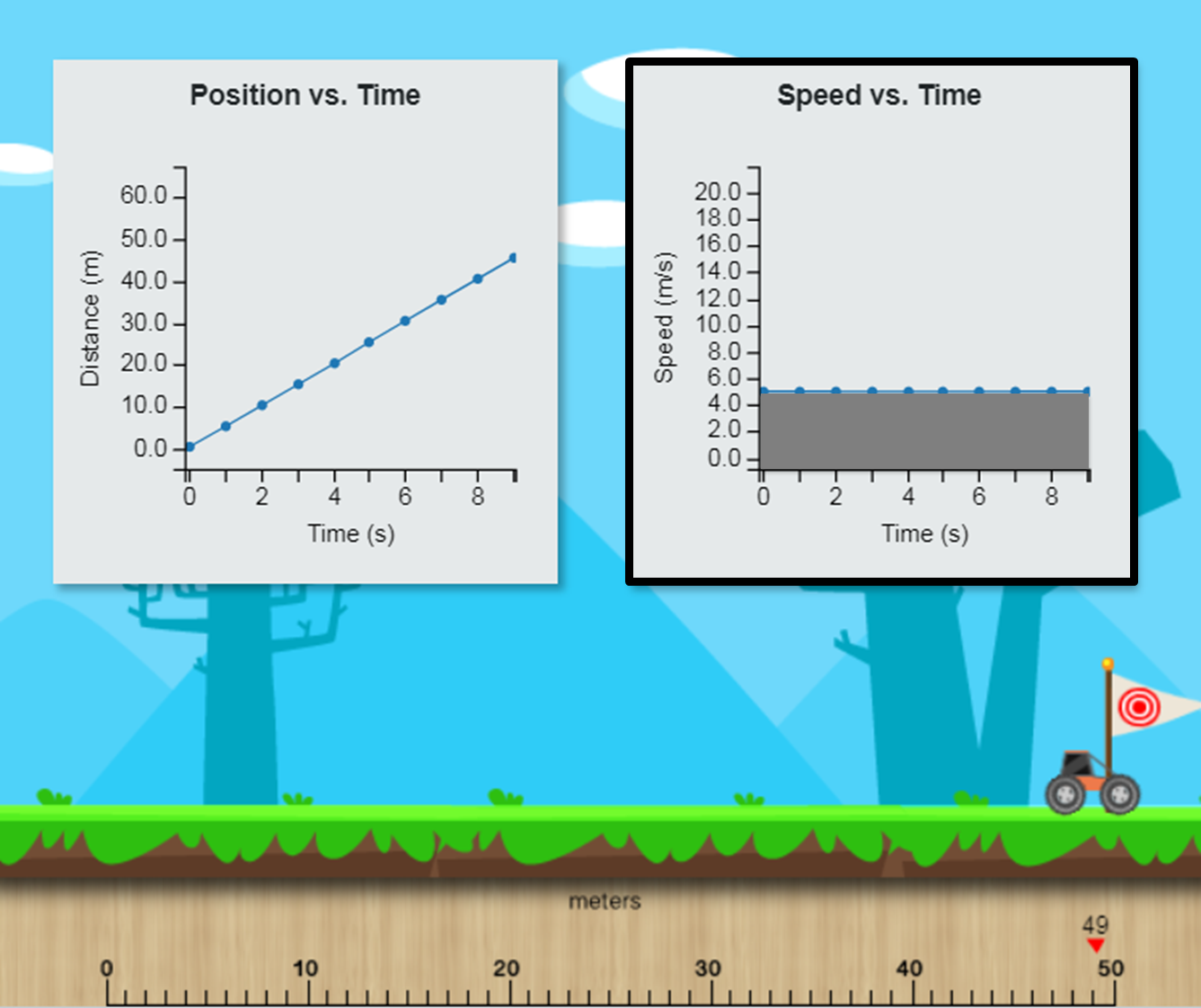
Example: Chart of a toy car

The following table shows the position of a toy car moving at a constant velocity. You can see the answer on the next page.

Time (s)	Position (m) [N]	$\vec{d}$
0	0	d
5	20	d₁
10	40	d₂
15	60	d₃
20	80	d₄

Plot a position-time graph for the motion of the toy car.

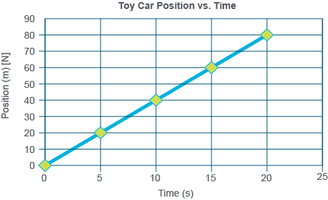
Determine the velocity of the toy car from the position-time graph.

$s l o p e = \frac{r i s e}{r u n}$

$m = \frac{80 m [N]}{20 s}$

$m = 4.0 m / s [N]$

The velocity of the toy car is 4.0 m/s [N].

Plot a velocity-time graph.

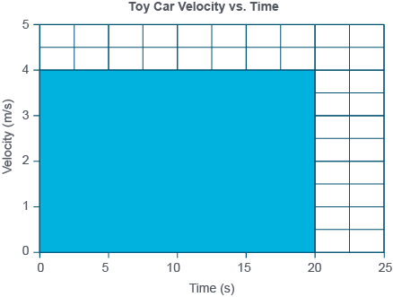
Represent displacement from 0s to 20s.

Determine the area between the velocity line on the velocity-time graph and the time axis for the time interval from 0 s to 20 s. This area corresponds to the displacement of the toy during the same time interval.

Area of shaded region in the previous image:

area = length x width

area = (4 m/s [N])(20 s)

area = 80 m [N]

To show that this area represents the displacement, use the position of the car at 0 s and 20 s (80 m [N]), as follows:

$\vec{∆ d} = \vec{d_{2}} - \vec{d_{1}}$

$\vec{∆ d} = 80 m [N] - 0 m [N]$

$\vec{∆ d} = 80 m [N]$

Understanding checkpoint

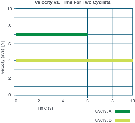
The v-t graph shows two horizontal lines in different colours, one at 7 m/s [S] labelled Cyclist A and the other at 4 m/s [S] labelled Cyclist B. Cyclist A’s line extends from 0 s horizontally to 6.0 s. Cyclist B’s graph extends horizontally from 0 s to 10 s.

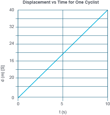
Chart with Cyclist A at 9 m/s for 6 seconds and Cyclist B at 4 m/s for 10 s

The d-t graph starts at (0 s, 0 m [S]) and extends upwards to the right to (10 s, 40 m [S]) in a straight line.

Displacement vs time. 10 s on horizontal axis, 40 m on vertical axis in a straight line

Newton’s first law of motion

Three laws of motion

Three laws of motion were described and published by Sir Isaac Newton (1643–1727) more than three centuries ago. These laws describe how and why things move the way they do. A summary of these laws is:

First law of Newton: An object in motion will continue to move and an object at rest will remain at rest until some outside force acts on it.

Second law of Newton: If the net force on an object is not zero, it will accelerate in the direction of the net force. The acceleration is directly proportional to the net force and inversely proportional to the mass.

Third law of Newton: For every action force there is a reaction force equal in magnitude but opposite in direction.

In the next few lessons, we will look at how these three laws are applied to everyday activities. Let’s start with the first of Newton’s laws of motion.

You’ve seen that motion is a continuing change of position. It is displacement that continues over time. You’ve also learned that uniform linear motion means moving in a straight line at a constant velocity. Let’s find out more about motion: what causes it, and how it can be changed.

Newton’s first law of motion states that:

An object in motion will continue to move and an object at rest will remain at rest until some outside force acts on it.

In other words, Newton showed that an object that has no outside forces acting on it will continue to move in a straight line at a constant velocity. Similarly, an object that is at rest will stay at rest until a force acts on it. This law is often paraphrased as follows: “If the net force acting on an object is zero, the object will maintain its state of rest, or if it is moving, it will continue to move with a constant velocity”.

Force

In the previous section, you learned that force is what causes a change in motion. Force is what can change the velocity of an object; it’s a push or a pull that starts, stops, or changes the uniform motion of an object. Let’s explore this concept in detail.

Force is what produces or prevents motion. Force is measured in Newtons (N).

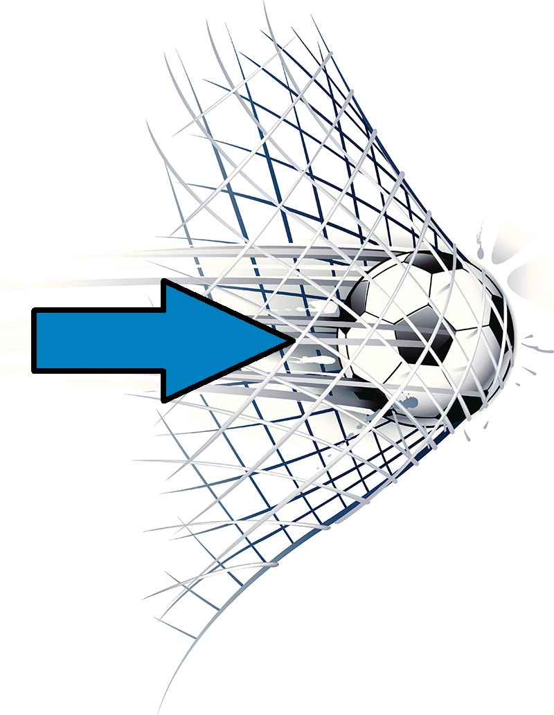
Soccer ball applying a force to a soccer net

When you lift a book from a table, kick a soccer ball, throw a stone, or stretch a rubber band, you are making objects move by applying a force — a push or pull. When you catch the book as it falls, or deflect the ball that’s headed at the net, you’re applying force to stop an object or change its direction.

In addition, force is a vector quantity. Like displacement and velocity, it has both magnitude and direction. When a force is applied to an object, the direction in which the object is pushed or pulled is called the direction of force.

Net force

Most objects have many different forces acting on them. In order to keep things simple, for this lesson, you will consider only the net force or total force acting on an object.

Net force (Fnet) is the sum of all the forces acting on an object and can be used in place of listing all of them. The object will react to this single net force in the same way as it would to all forces simultaneously acting on it.

Implications of the first law of motion

Newton’s first law leads to several implications, including the following:

Objects at rest

Objects at rest will remain at rest unless acted upon by a net force
If an object is at rest, the velocity of the object is zero, and the net force acting on the object must be zero
If an object is at rest and it starts to move, the change must be caused by a net force acting on the object

Objects in motion

Objects moving with a constant velocity will continue to move with a constant velocity unless acted upon by a net force
If an object is in uniform linear motion, the velocity of the object is constant, and the net force acting on the object must be zero
If the velocity of an object is changing in magnitude or direction or both, the change is caused by a net force on the object

Now that you know something about the concept of force and the implications of the first law of motion, you are ready to analyze different scenarios concerning what kind of forces are acting on the objects, what effect they have, and how they relate to Newton’s first law of motion.

Scenarios

Scenario 1: A car on an icy road

A car is moving along a straight section of road covered in very slippery ice. Under normal circumstances when a driver applies the brakes, they transmit the force to the tires using friction, and the tires transmit that force to the road also using friction.

The force of friction from the tires stopping on the road slows the car down. When the road is covered in ice, however, it is smooth and slippery, so there is less friction between the tires and the road. When a driver applies the brakes, they will notice the car doesn’t slow down as it normally would. In fact, it continues to move at the same velocity as it was travelling before. It continues moving with uniform motion. Since the surface is iced, it is smooth and there is no friction from the road to slow the car down. No net force is being applied to stop the car, so it will continue to move at a constant velocity until it either hits an object or makes its way over the ice and on to a non-icy part of the road.

You can see what happens in this video when friction between the road and tires of the car is lost.

Scenario 2: Galileo’s experiment

Galileo was an Italian physicist, mathematician, astronomer, and philosopher who came up with a simple experiment nearly four centuries ago. His “thought experiment” is illustrated in the following images.

a) If friction could be eliminated...

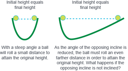
b) If friction could be eliminated...

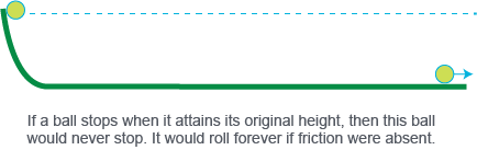
You can also see his reasoning in the following video:

To do this experiment, you need to pretend that a ball can move across a surface and experience no friction at all. If that were the case, then in situation (a) the ball would roll down the first incline, across the level surface, and then up the second incline until it reached the same height. If the steepness of the second incline were reduced, the ball would have to roll farther to reach the same height. Galileo concluded that if there were no second incline, as in situation (b), the ball would continue to move forever in the absence of friction since it would never reach the same height. Galileo referred to this property of matter as inertia. Inertia causes matter to resist changes in motion. In the example, the ball shows the property of inertia because it keeps moving with uniform motion unless a force makes it change its motion—it resists a change in motion. Similarly, an object at rest will remain at rest unless a force causes it to move—it too resists a change in motion. Newton used Galileo’s ideas when he developed his first law of motion.

Scenario 3: Seat Belt

Watch the following video:

In a car accident, if a person is not wearing a seat belt, they can be severely injured. In a seat belt, the strap exerts a force on the person and helps slow the person’s motion as the car slows down. The stopping force of the seat belt can help prevent injury.

Seat belt under normal conditions

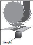
The seat belt strap or webbing is typically wrapped around a sprocket that is free to rotate either way to provide enough give and take for a person to sit comfortably.

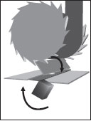
Seat belt when the car stops suddenly

A pendulum attached to a lock bar swings forward because it continues to move forward at a constant velocity (Newton's first law).

The forward motion of the pendulum causes the lock bar to swing back and forces it into the teeth of the sprocket. With that, the sprocket is locked and cannot rotate. The locked sprocket grips the strap of the seat belt so it cannot loosen any further. The locked strap exerts a force on the person, which stops the forward motion. The person is held in the seat by this force instead of continuing the uniform motion into the windshield.

The following video may help explain the action of a seat belt:

Understanding checkpoint

Discuss each of the following statements, using Newton’s first law to support your comments:

It is dangerous to store heavy or sharp objects in the rear window space of a car.

Student Answer

According to Newton’s first law, if the car stops suddenly, the objects stored in the rear window space will continue to move forward at a constant velocity and they could hit people inside the car from behind.

You should slow down when a road is covered with ice.

Student Answer

According to Newton’s first law, when the driver applies the brakes, there is little (if any) friction acting on the car and the car continues to move at a constant velocity. This, of course, could cause an accident.

Portfolio

Congratulations! You have almost reached the end of this lesson.

At the end of every lesson, you will be asked to complete a wrap-up assignment, which will be part of your course Portfolio. You will then submit this Portfolio at the end of the course for marking. Refer to the Communication Guidelines (Opens in new window) for more information about typing responses to math and science questions.

Instructions:

Step 1: Create a new file using Word, Google Docs, or another word processor. Save it in a place you can find later. This file will contain your responses to the portfolio entries at the end of each lesson.

Step 2: Save “Learning Activity 1.1 portfolio (Opens in new window)” for the assignment corresponding to this lesson.

Step 3: Add a title to your Portfolio document to show that you are responding to the Learning Activity 1.1 portfolio entry. Remember to add a title for each new portfolio entry. You can also choose to stay organized by starting a new page for each new entry (along with a title). Remember to re-save your portfolio document when adding new entries.

Step 4: Always back up your work!

At the end of your course, you will write a Final Test. Completing the Portfolio is an excellent review in preparation for the Final Test. The Portfolio will also help you to keep track of important knowledge and skills that you have gained throughout the course. Each of the Portfolio Assessments will have a summative grade.